Functionality of Predictive Coding

Mentor: Mazen Al Borno

"There is nothing so practical as a good theory." — Kurt Lewin

What is Predictive Coding?

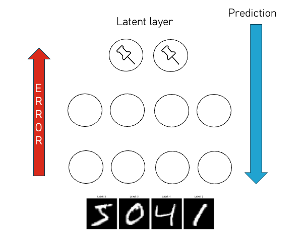
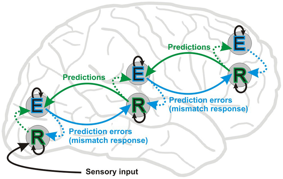Predictive Coding overview diagram

Predictive Coding is a biologically inspired neural network framework built on a simple but powerful idea: the brain does not passively process sensory information. Instead, it continuously forms a prediction of what the sensory input will be, then updates itself based on the error between prediction and reality.

This happens in a localized, hierarchical manner:

Top-down: predictions flow downward through the hierarchy
Bottom-up: prediction errors flow upward

The framework was first theorized by Rajesh Rao and Dana Ballard in 1999 and has since become a foundational model in computational neuroscience.

Stefanics G, Kremláček J and Czigler I (2014) Visual mismatch negativity: a predictive coding view. Front. Hum. Neurosci. 8:666. doi: 10.3389/fnhum.2014.00666

The Free Energy Principle

Any self-organizing system that is at equilibrium with its environment must minimize its free energy [Surprise]. The principle is essentially a mathematical formulation of how adaptive systems resist a natural tendency to disorder. — Karl Friston

The Free Energy Principle, introduced by Karl Friston, provides the mathematical backbone for Predictive Coding. "Free Energy" in this context is a proxy for surprise — the degree to which incoming data deviates from the model's expectations.

The brain is constantly making predictions about what it expects to see. When reality matches the prediction, the prediction error is low, free energy is minimized, and the brain largely ignores the input — it's nothing new.

A normal upright chair — exactly what the brain expects

Take a chair sitting normally on the floor. Your brain has seen thousands of chairs. It has a strong, well-calibrated internal model: four legs, upright, seat on top. When you walk into a room and see this, the prediction error is essentially zero. Your model said "chair, upright" and that's exactly what arrived. Low surprise. Low free energy. The brain moves on.

Now consider this:

A chair tipped and rotated at an odd angle — high prediction error

The same chair, but knocked over and rotated at an awkward angle. Your brain's model predicted "chair, upright" — what it received was something that barely matches. The prediction error spikes. Free energy rises. The brain is forced to pay attention, update its belief about what it's seeing, and reconcile the mismatch.

This is the core mechanism: the brain doesn't process everything equally. It is a prediction machine that filters the world through its own expectations. Unsurprising things get suppressed. Surprising things — things that violate the model — demand resources and drive learning.

A system minimizes free energy (surprise) by one of two means:

Update the internal model — change what you expect so the prediction improves (learning)
Act on the environment — change reality to match the prediction (action)

Friston, K. The free-energy principle: a unified brain theory?. Nat Rev Neurosci 11, 127–138 (2010). https://doi.org/10.1038/nrn2787

In a Nutshell

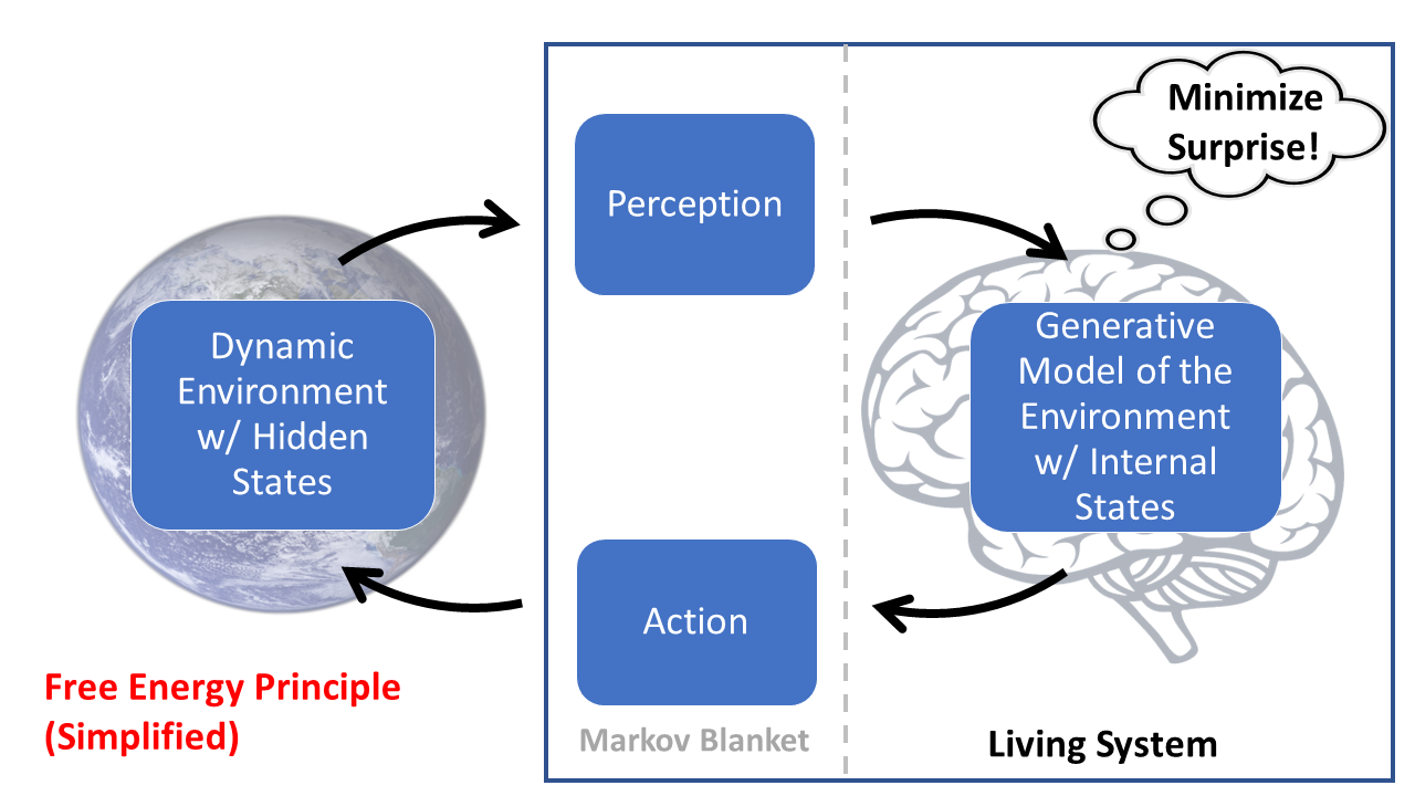Free Energy principle simplified

How it Differs from Deep Neural Networks

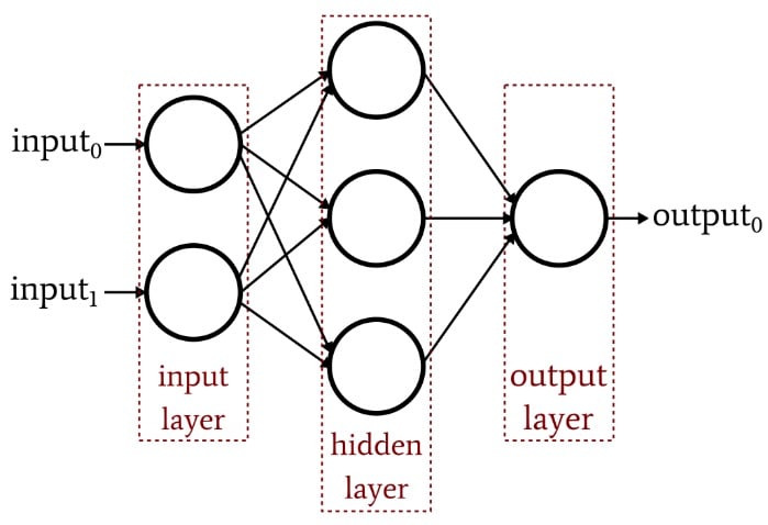Deep Neural Network vs Predictive Coding comparison

Standard deep neural networks operate in two phases:

Forward pass — compute output from input
Backpropagation — propagate a global error signal backward to update weights

Predictive Coding is different in a fundamental way. There is no separate forward and backward pass. Instead, the network simultaneously maintains:

Predictions flowing top-down
Errors flowing bottom-up

Updates happen locally and iteratively, not via a global backprop signal. This makes PC networks more biologically plausible and opens the door to running on neuromorphic hardware.

The Foundation

The core loop of a Predictive Coding network:

State → Belief — the network forms an internal belief (prediction) based on its current state
Prediction Error — the error between prediction and actual input is computed
Iterative Update (ΔW) — weights are updated to minimize Free Energy (surprise)

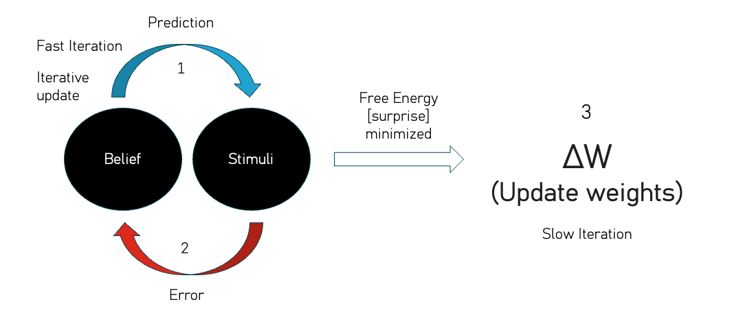Predictive Coding foundation diagram — Belief, Stimuli, Prediction, Error, and weight update loop

This runs on two timescales:

Fast iteration — inference: the network self-organizes to express its current belief
Slow iteration — learning: weight updates that shift the model over time

Interacting with a Predictive Coding Network

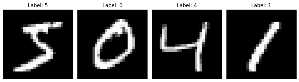Predictive Coding network architecture

A Predictive Coding network has two key mechanisms:

Inference loop — Before learning, the network must self-organize to express a belief. It iteratively adjusts its internal prediction until free energy is minimized. This is the "settling" phase.

Clamping — PC networks learn on demand. To have the network form a belief, either the top layer or the bottom layer is pinned (clamped) to data. Different clamping combinations produce different behaviors:

Clamped Layer	Behavior
Bottom (input) only	Unsupervised autoencoding
Bottom + Top	Supervised classification
Top (latent) only	Generative sampling

Unsupervised: Autoencoder

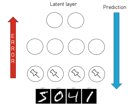Autoencoder clamping diagram — bottom layer pinned to input digits, error flows up, prediction flows down

In autoencoder mode, the bottom layer is clamped to the input and the network is left to find a compressed internal representation that minimizes reconstruction error.

Autoencoder Results

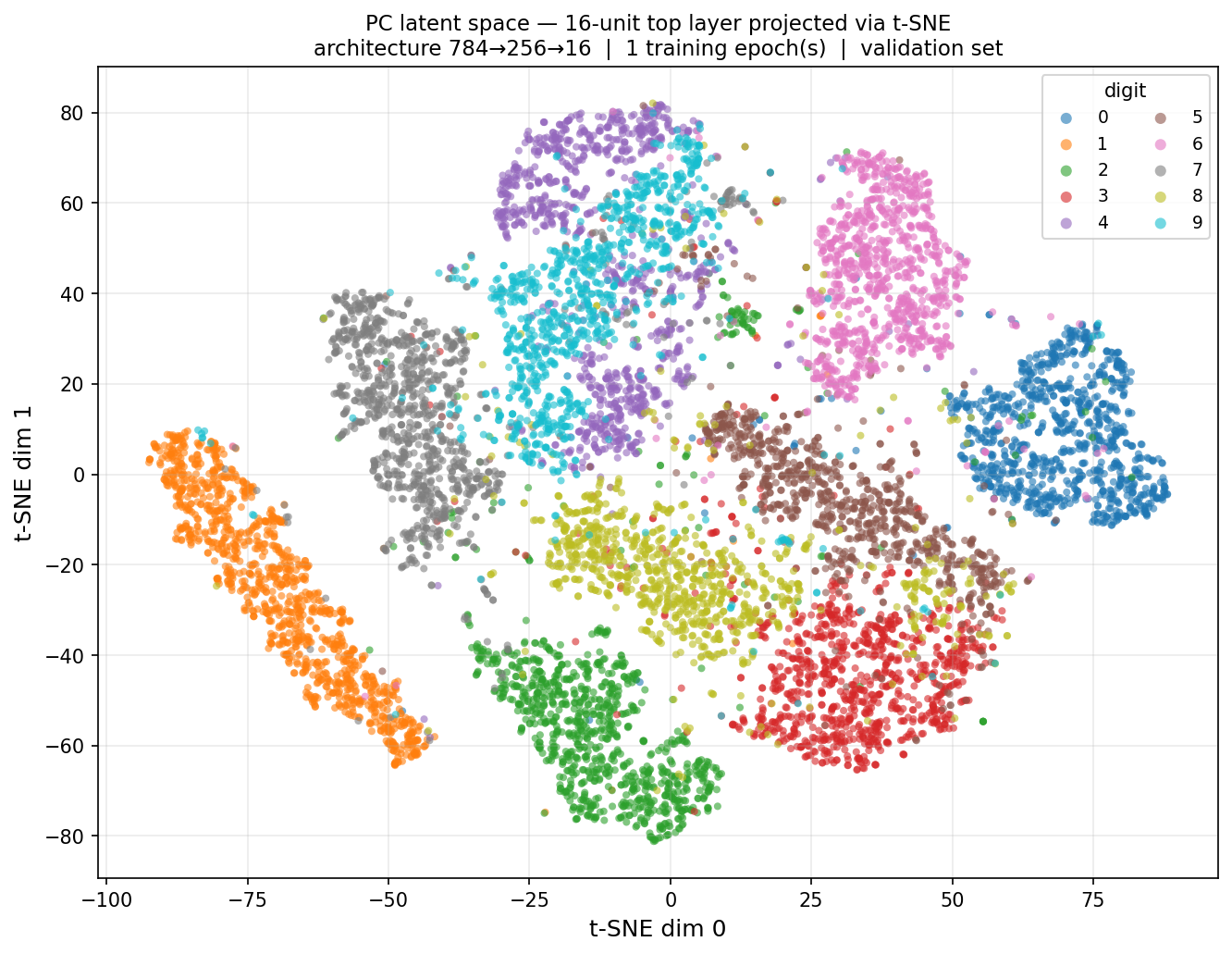Autoencoder t-SNE results

Setup: 1 epoch, 16-unit top layer, t-SNE used to reduce the latent space to 2D for visualization.

Result: Digits with similar visual structure cluster together in the learned latent space. Notably, 4 and 9 are close to each other, forming a split cluster — which makes intuitive sense given their structural similarity.

Supervised: Classifier

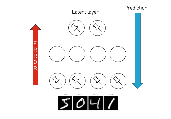Supervised classifier — both input and latent layer pinned, error flows up, prediction flows down

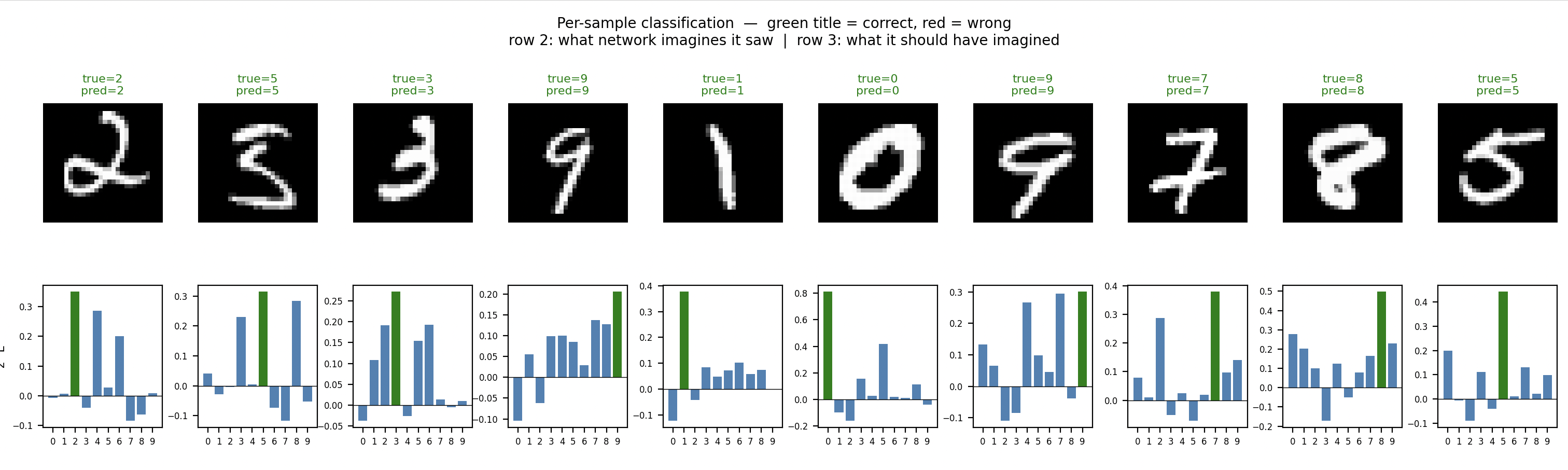
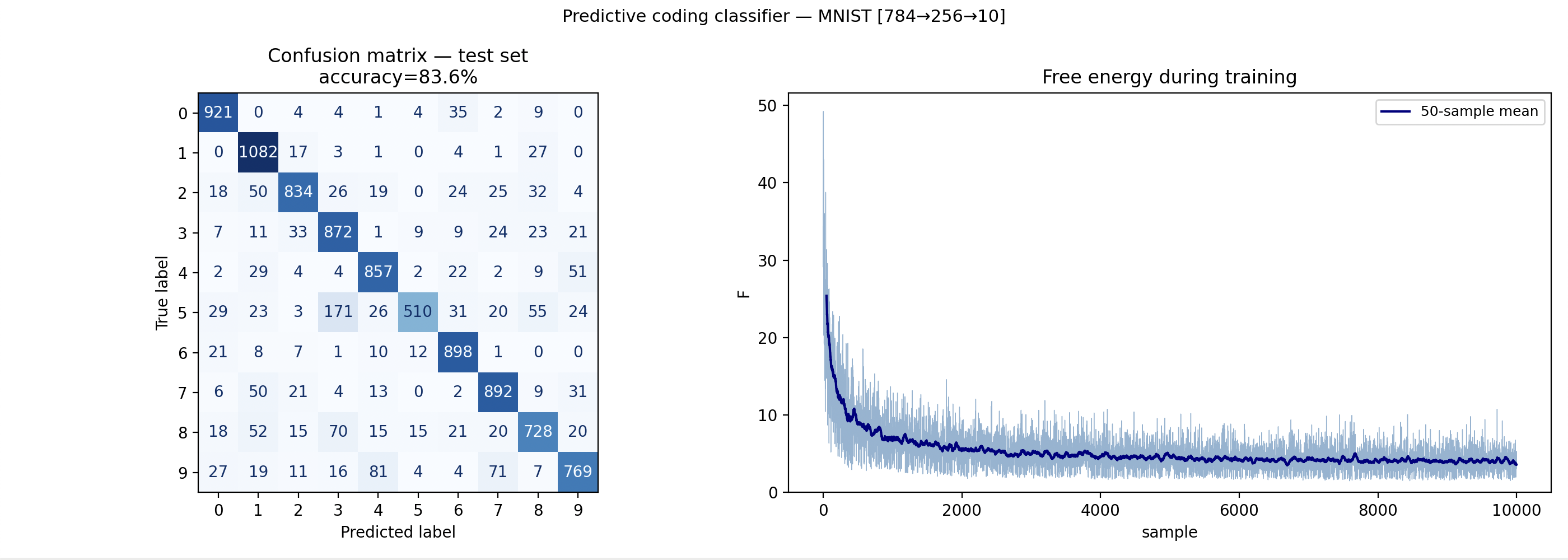
In classifier mode, both the input (bottom) and the label (top) are clamped during training. At inference, only the input is clamped and the network infers the most likely label.

Classifier Results

Classifier results

Classifier results detail

Generative Mode

Generative mode — only the latent layer is pinned, prediction flows down to synthesize output

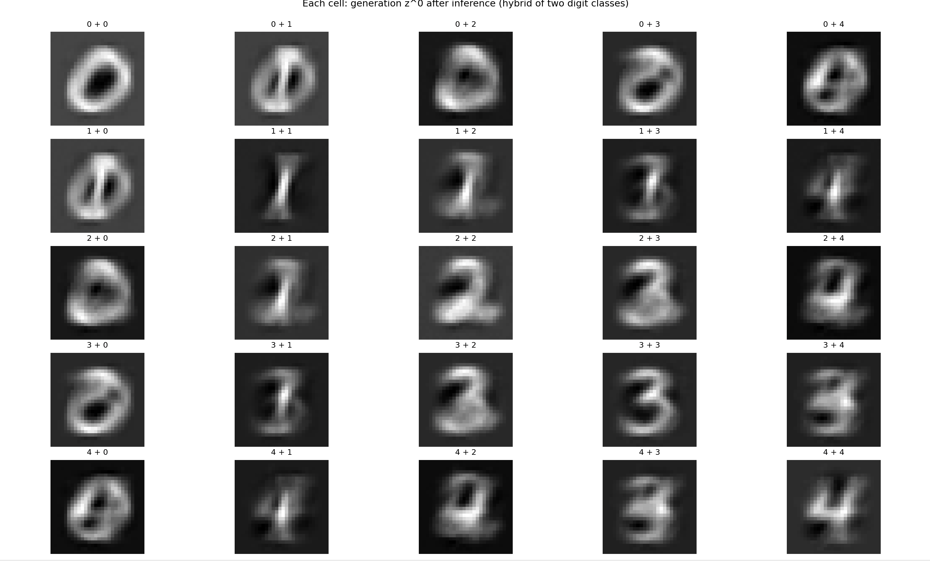
In generative mode, only the top (latent) layer is clamped. The network propagates predictions downward to synthesize an output consistent with the given latent state.

Generative Results

Generative results

Generative results detail

Mapping to Spiking Neural Networks (SNN)

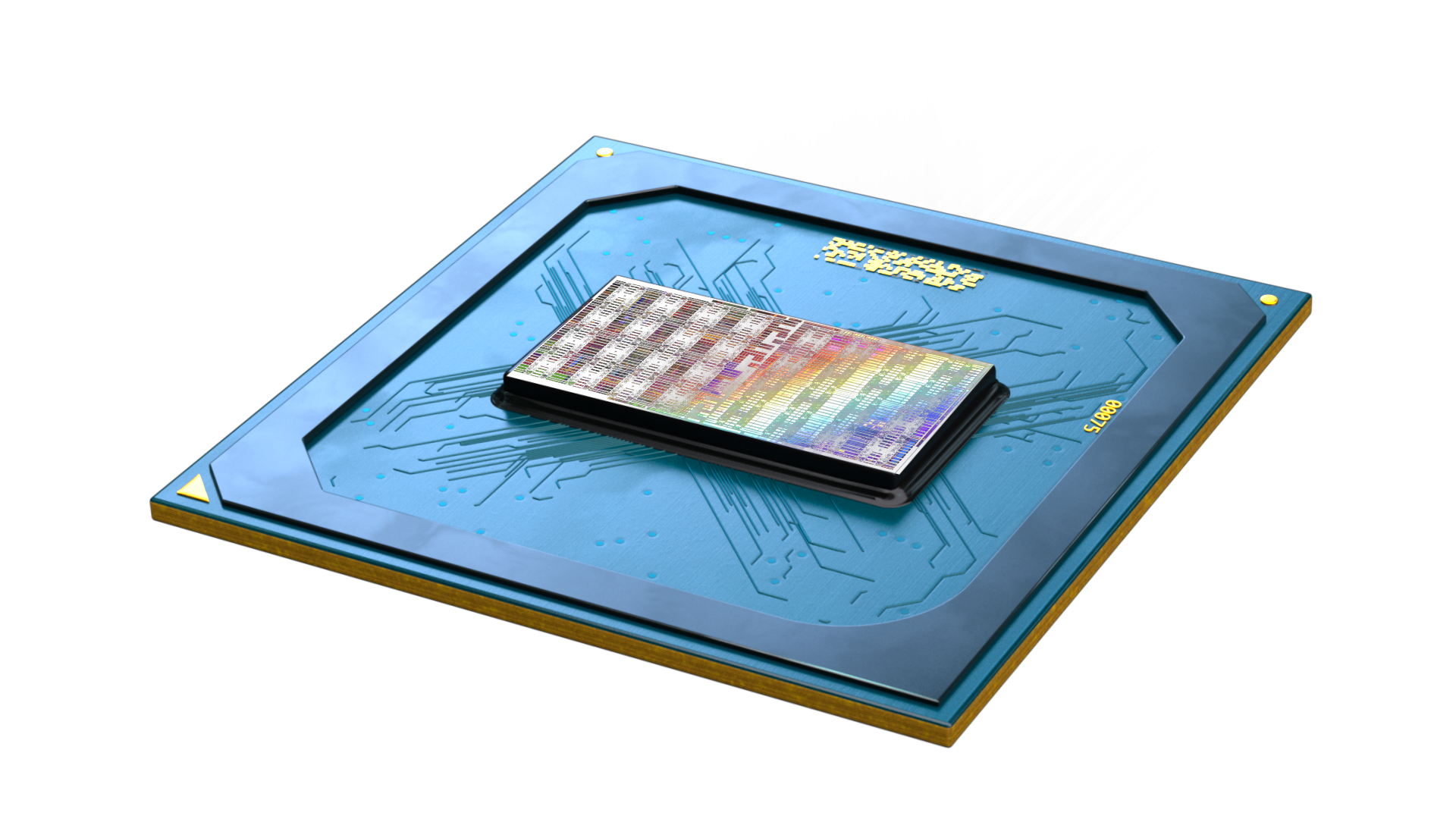PC mapped to Spiking Neural Network on Loihi 2

"Predictive Coding uses Hebbian learning rules local enough to be exportable to SNN."

One of the most compelling properties of Predictive Coding is that its weight updates depend only on pre- and post-synaptic activity — no non-local error signals are needed, unlike backpropagation. This makes it a natural fit for Spiking Neural Networks and neuromorphic hardware.

The PC-SNN uses a 3-factor local learning rule: pre-synaptic spike, post-synaptic spike, and a modulatory signal — triggering updates only when and where spikes occur. This event-driven sparsity is exactly what neuromorphic chips like Intel Loihi 2 are purpose-built to exploit.

The results are striking:

70× faster inference
5,600× more energy efficient

Hajizada et al. (2025). Real-time Continual Learning on Intel Loihi 2. arXiv:2511.01553v1

Predictive Coding Continuously Learns

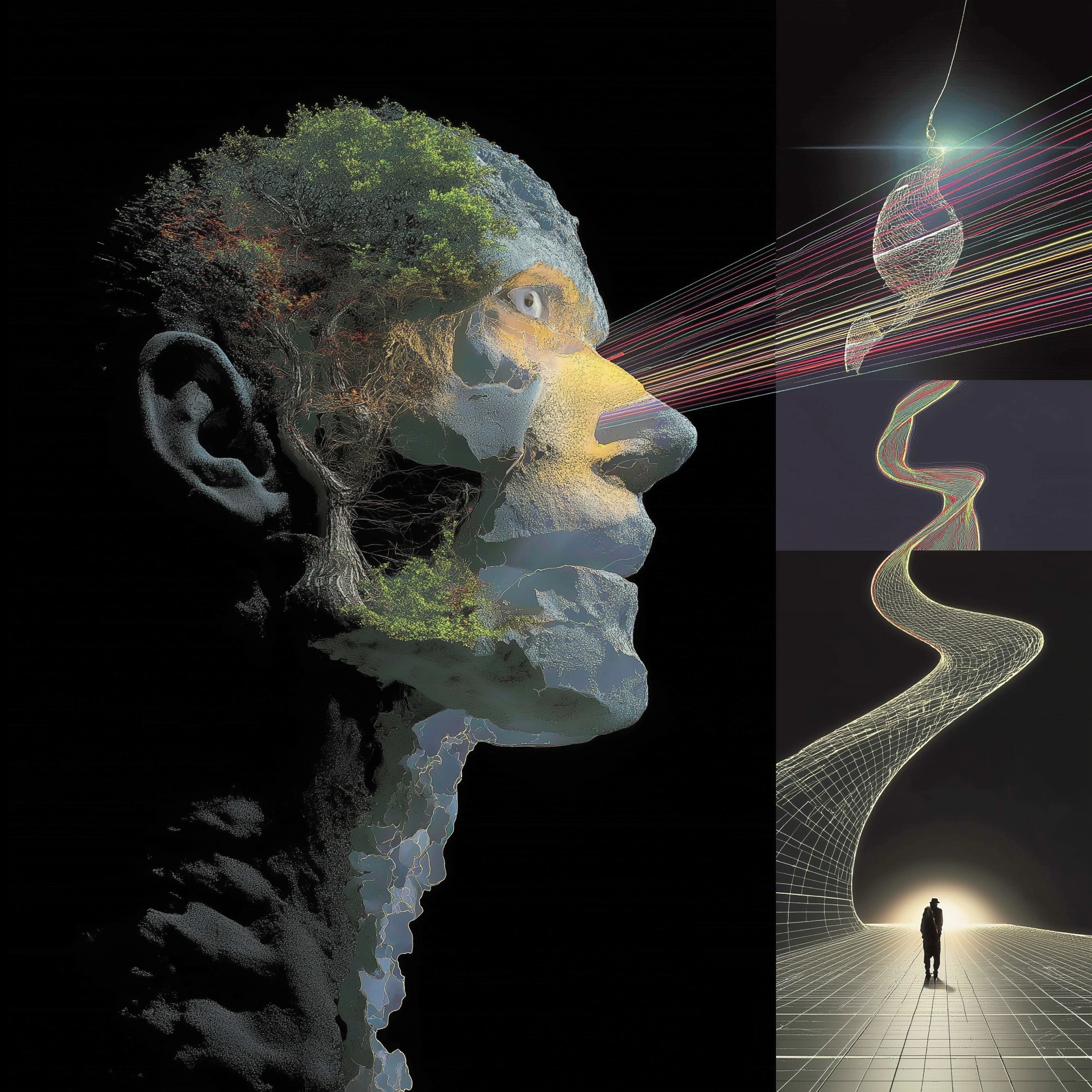Continual learning diagram

"In a real-world environment there is no need to retrain when the distribution changes."

Standard deep learning assumes training and deployment distributions are identical — this breaks down in open-world settings. Predictive Coding networks do not have this limitation. Key properties that enable true continual learning:

Meta-plasticity — each prototype's learning rate adjusts based on correctness: stable memories resist overwriting, plastic ones update readily
Neurogenesis — new neurons are allocated on demand when novel concepts are encountered, expanding capacity without retraining
No rehearsal buffer needed — unlike replay-based methods, prior knowledge is retained without storing old data

Hajizada et al. (2025). Real-time Continual Learning on Intel Loihi 2. arXiv:2511.01553v1

Presentation

This work was presented at the 2026 RACAS Symposium. You can view the full presentation entry here:

2026 RACAS Symposium — Functionality of Predictive Coding

References

Rao, R. P. N., & Ballard, D. H. (1999). Predictive coding in the visual cortex. Nature Neuroscience, 2(1), 79–87.
Friston, K. (2010). The free-energy principle: a unified brain theory? Nature Reviews Neuroscience, 11(2), 127–138. https://doi.org/10.1038/nrn2787
Friston, K., & Kiebel, S. (2009). Predictive coding under the free-energy principle. Phil. Trans. R. Soc. B, 364(1521), 1211–1221.
Bogacz, R. (2017). A tutorial on the free-energy framework for modelling perception and learning. Journal of Mathematical Psychology, 76, 198–211.
Bastos, A. M., et al. (2012). Canonical microcircuits for predictive coding. Neuron, 76(4), 695–711.
N'dri, A. W., et al. (2024). Predictive coding with spiking neural networks: A survey. arXiv:2409.05386.
Hajizada, E., et al. (2025). Real-time continual learning on Intel Loihi 2. arXiv:2511.01553.
Tscshantz, A., et al. (2023). Hybrid predictive coding: Inferring, fast and slow. PLOS Computational Biology, 19(8), e1011280.